
Why I built this
I was halfway through my master’s when I realised I didn’t actually understand fine-tuning. I could call trainer.train(). I could read a loss curve. I could tell you the difference between LoRA and full fine-tuning at a cocktail-party depth. But if you’d asked me to explain why low-rank adaptation works — what the rank actually constrains, why some target modules matter more than others — I’d have hand-waved you through it and hoped you didn’t follow up.
So I went looking for something that would close the gap. I read papers. I watched courses. I ran a dozen tutorials. Half of them assumed I already knew the maths and just walked me through API calls. The other half wrapped everything in a hosted notebook with a button that said “Run cell” and skipped the maths entirely. Nothing I found taught the intuition and the code together in a way that respected the fact that I wanted to understand what I was running, not just watch it run.
So I built what I wanted to read. Nineteen lessons across nine modules, each one in three formats — a long-form markdown explanation, a clean Python script, and a runnable notebook. Every script generates its own synthetic data and runs on a laptop. I’m publishing it because the next person learning this shouldn’t have to start where I started.
The four design principles
Self-contained. No API keys, no cloud accounts, no external datasets. The single biggest reason fine-tuning tutorials fall over is that the dataset link rots, the API quota expires, or the notebook assumes a paid runtime. Every lesson here generates its own synthetic data and runs end-to-end on whatever machine you already own. The friction between “I want to learn this” and “I’m seeing a result” is as close to zero as I could make it.
Concept first, code second. Every lesson opens with the theory — the maths, the trade-offs, the analogies, the ASCII diagrams — and only then introduces code. This was the principle I worked hardest on. The temptation when writing a fine-tuning lesson is to lead with from peft import LoraConfig and explain as you go. I forced myself to do the opposite: explain what a low-rank decomposition is, why it works as an approximation, what you’re giving up in exchange for the parameter savings — and only then write the line that imports the library.
Three formats per lesson. Markdown for reading, Python script for skimming the clean code, Jupyter notebook for running cell-by-cell. The three formats aren’t redundancy. They map to three different learning modes — reading to understand, running to see, and editing to internalise — and I wanted each lesson to support all three without asking the learner to context-switch between sources.
Small models, real patterns. Every lesson uses a model between 60M and 124M parameters — distilbert-base-uncased, bert-base-uncased, gpt2, t5-small. You can train all 19 lessons on a CPU. The point isn’t that you’d fine-tune a 66M-parameter encoder in production; the point is that the patterns — LoRA, QLoRA, DPO, the SFTTrainer pipeline — are identical at 66M and at 70B. Learn them on something that fits in your laptop’s RAM, then apply them where they need to go.
What’s in the course (at a glance)
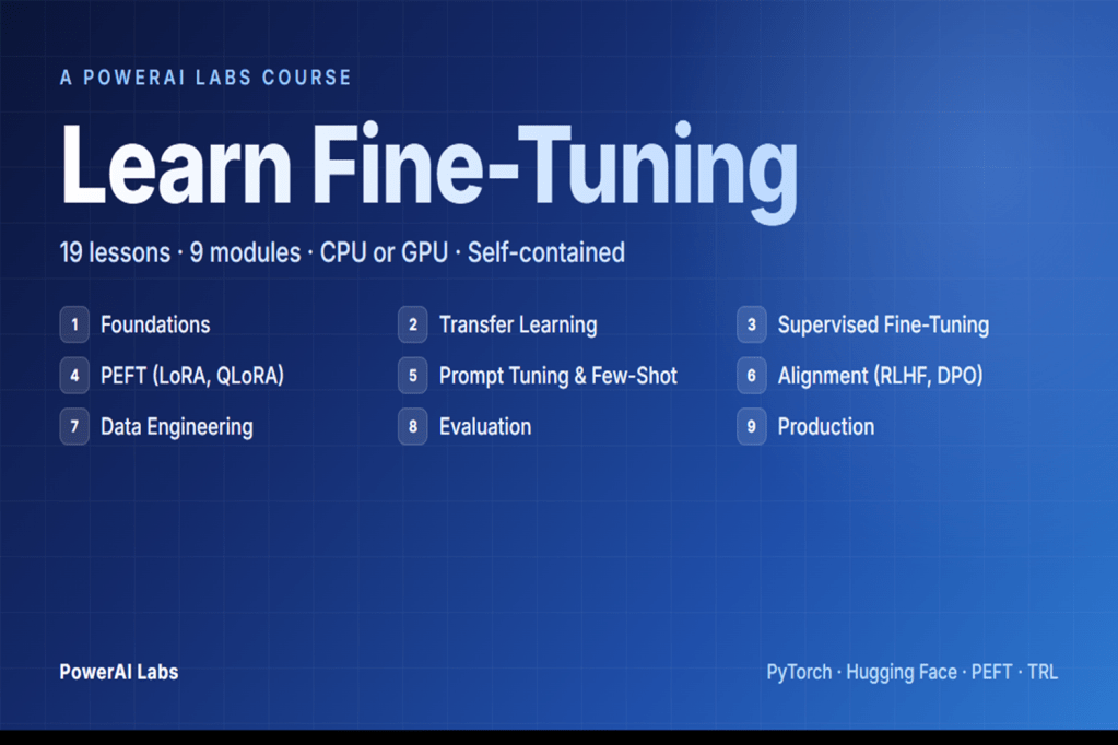
The shape of it: foundations → transfer learning → supervised fine-tuning → PEFT (LoRA, QLoRA) → prompt tuning and few-shot → alignment (RLHF, DPO) → data engineering → evaluation → production. Nine modules, nineteen lessons, each one building on the last.
I’m deliberately not walking through them one by one here — that’s what the Project page on PowerAI Labs is for, and the repo README has the full lesson-by-lesson breakdown with topics, models, and the papers behind each one.
The three things I learned that surprised me
LoRA’s rank is less sensitive than the papers suggest — but the target modules are everything
I expected rank to be the lever I’d spend the most time tuning. It isn’t. On the tasks I worked through in the course, rank 4, rank 8, and rank 16 produced results that were within noise of each other. Above rank 16 the gains were small enough that I struggled to justify the extra parameters; below rank 4 the model would start to underfit, but the transition wasn’t dramatic.
What did matter, by a long way, was which modules the LoRA adapters were attached to. Adapting only q_proj left obvious capacity on the table. Adapting q_proj and v_proj — the original LoRA paper’s recommendation — was a meaningful step up. Adapting all linear layers was a further step up again, at a parameter cost that was still tiny relative to full fine-tuning. The rank-vs-target-modules trade-off is the one I now reach for first when a LoRA run isn’t doing what I want, and it’s the opposite of what I’d have guessed before I built the course.
DPO is genuinely simpler than RLHF, and the implicit reward is the real insight
I’d read the DPO paper before I built Module 6, and I thought I understood it. I didn’t, not properly. The insight that survives once you’ve worked through both a full RLHF pipeline and a DPO pipeline back-to-back is that DPO doesn’t replace the reward model — it absorbs it. The Bradley-Terry preference equation can be rearranged so that the reward score is expressed as a log-ratio of policy probabilities to a reference policy, and once you make that substitution the entire reward-model-then-PPO machinery collapses into a single supervised loss over preference pairs.
The practical consequence is that DPO is dramatically less code than RLHF, has no reward-model overfitting failure mode, and trains stably with a single hyperparameter — beta — that you can actually reason about. The conceptual consequence is harder to express but more important: once you see that the reward signal is implicit in the policy itself, you start to see alignment as a property of the model rather than a separate system bolted on top. You cannot unsee it.
Quantisation and PEFT compose better than I expected
QLoRA’s claim — fine-tune a billion-parameter model on a single consumer GPU at near-LoRA accuracy — sounded like marketing. It isn’t. In the lessons where I ran the comparison properly, QLoRA was within a percentage point of standard LoRA on the same task at a fraction of the VRAM. The two ideas — 4-bit NF4 quantisation of the base model, low-rank adaptation on top — compose almost orthogonally, and you genuinely lose very little to the quantisation when the adapters are doing the work.
The practical implication isn’t subtle. Production-ready LoRA fine-tuning on a single consumer GPU is real, today, with the libraries on the install list at the top of the course. That was true in research a year ago and it’s true on a laptop now, and it changes the economics of what an individual engineer can do without asking finance for a cluster.
Who this is for
For engineers who want to learn by running code. For architects who need to understand what the abstractions hide before they sign off on a design that depends on them. For master’s students working on adjacent topics who want a concrete codebase next to the papers. For anyone who has felt the gap between “the code works” and “I understand what it did” and wants to close it.
Not for people who want to call an API and move on — there are great products for that, and you don’t need this course to use them. Not for people who want a polished, certificate-bearing online course with video lectures and a discussion forum. This is self-paced, open-source, and rough-edged. The rough edges are part of the learning.
What’s next
The course lives at its Project page on PowerAI Labs, with the code on GitHub. Clone it, star it, fork it, file issues with corrections — I read every one, and corrections from people working through the material are the single best signal I get on what to tighten next.
Over the next few months I’ll publish a deep-dive blog post per module on PowerAI Labs, starting with LoRA — the rank-versus-target-modules result above is going to need its own post to do it justice. Subscribe if that’s useful and I’ll link them here as they go live.

Leave a comment